Histogram maker.
Upload a CSV or Excel file, or paste your data. Choose the columns to plot, preview your histogram, and download it free.
Preview your histogram
Values are grouped into bins. You can adjust the bin settings below.
Blueprint styleDownload your chart
PNG for slides · SVG for editing · PDF for printing
Calculated values
Bins include their lower boundary; only the last bin includes its upper boundary.
| Lower boundary | Upper boundary | Count | Percent |
|---|---|---|---|
| 40 | 50 | 2 | 10 |
| 50 | 60 | 3 | 15 |
| 60 | 70 | 4 | 20 |
| 70 | 80 | 5 | 25 |
| 80 | 90 | 4 | 20 |
| 90 | 100 | 2 | 10 |
Inspect every input row (20)
| Score |
|---|
| 42 |
| 48 |
| 52 |
| 56 |
| 58 |
| 61 |
| 63 |
| 66 |
| 68 |
| 70 |
| 72 |
| 74 |
| 76 |
| 78 |
| 81 |
| 83 |
| 85 |
| 88 |
| 92 |
| 97 |
How to make a histogram
Group individual numeric observations into equal-width intervals. Choose a bin count or explicit start and width, inspect every frequency, and switch between counts and percentages.
- Upload a file or paste spreadsheet cells. Choose the columns and check the preview before creating your chart.
- Inspect every selected row. Missing or invalid numbers need correction; they are never filled with zero.
- Set the calculation options, then inspect the calculated values below the chart.
- Edit the title, labels and source note. Download an image, PDF, original CSV or ECharts configuration.
The editor accepts up to 2,000 observations for distributions and scatter plots, eight box-plot groups, or 50 bar/Pareto categories. A bar chart can include up to five series. Spreadsheet preview accepts files up to 8 MB, 2,000 rows and 100 columns. Data stays in your browser.
Choose the grouping deliberately
A histogram counts individual observations inside numeric intervals. Use the bin-count control for an initial equal-width partition, or enter a start and width for boundaries you can explain. Entering a width overrides the count. The chart supports at most 50 bins; it asks you to increase width when the requested range would exceed that limit.
Know which bin contains a boundary
Intervals include their lower boundary and exclude their upper boundary. The final interval includes both ends so the maximum observation is retained. With boundaries 0, 5, 10 and 15, an observation of 5 belongs in the 5–10 interval, and 15 belongs in the last interval. Inspect the calculated table to verify counts.
Counts, percentages and density differ
Count mode shows the number of observations in each bin. Percentage mode divides every bin count by the total observation count and multiplies by 100. It is relative frequency, not probability density. Because every interval has the same width, equal horizontal widths accurately represent equal numeric spans.
Read a summary without losing the source
All observations remain in the downloadable input CSV, including repeated values, negative numbers and genuine zeros. A histogram can hide small groups or gaps when bins are wide. Try another justified width before describing a shape, and use the dot plot maker when a small sample needs every value visibly separated.
Method references
Built by SupaMakers. Inspect the open source calculations and reuse terms.
Worked histogram examples
Explore the collection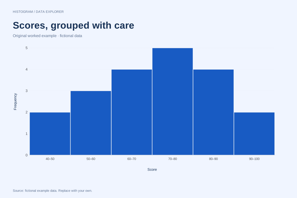
Histogram of class scores with ten-point bins
This histogram groups twenty fictional scores into ten-point intervals from 40 to 100. The count in each interval makes the concentration easier to compare while the downloadable list preserves every original score.
Explore chart & data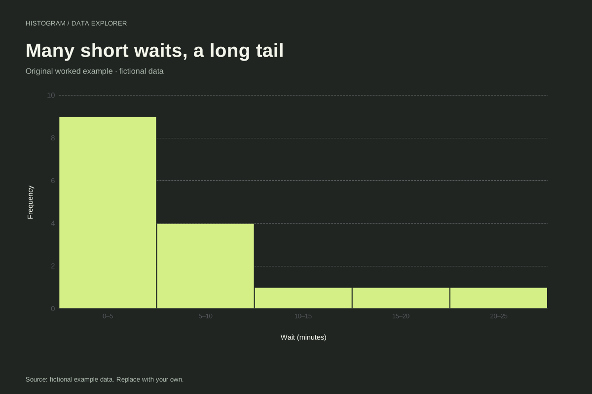
Right-skewed waiting-time histogram
This waiting-time histogram shows a concentration of short waits and a tail toward longer durations. Sixteen fictional observations are grouped into five-minute bins, making both the main cluster and the long waits visible.
Explore chart & data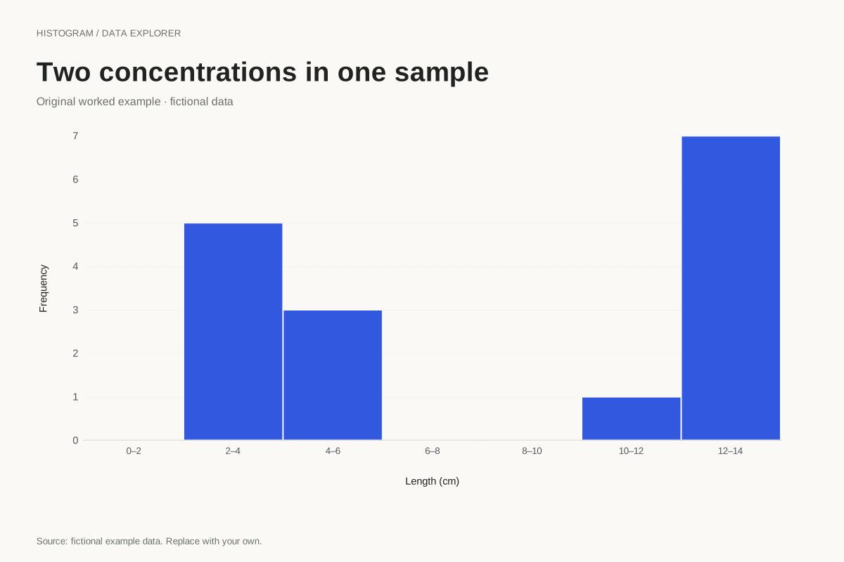
Bimodal histogram example with a gap
This constructed histogram places two clusters of fictional lengths on one numeric scale. The groups lie around 2–5 cm and 11–14 cm, separated by empty intervals that stay visible in the chart.
Explore chart & data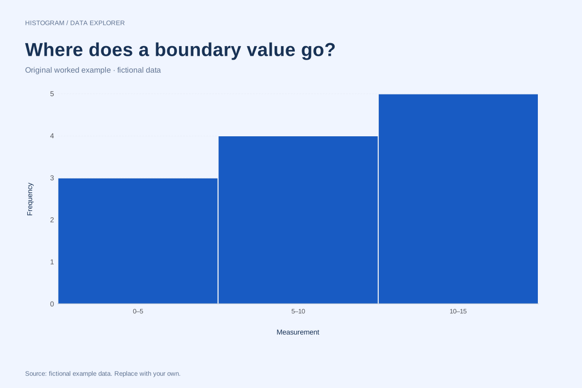
Histogram bin boundaries: where exact endpoints go
A value on a bin boundary must be assigned once. This twelve-observation example makes the boundary convention visible by placing repeated values exactly at 5 and 10, with a final observation at 15.
Explore chart & data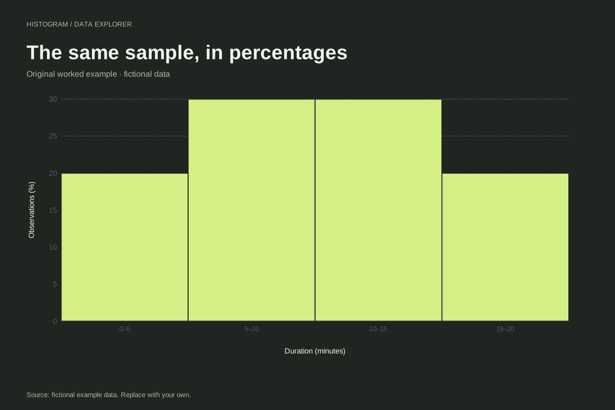
Relative frequency histogram with a worked percentage table
A relative frequency histogram expresses each bin count as a share of all observations. Here twenty fictional values become four bars of 20%, 30%, 30% and 20%, preserving the shape of the count histogram.
Explore chart & data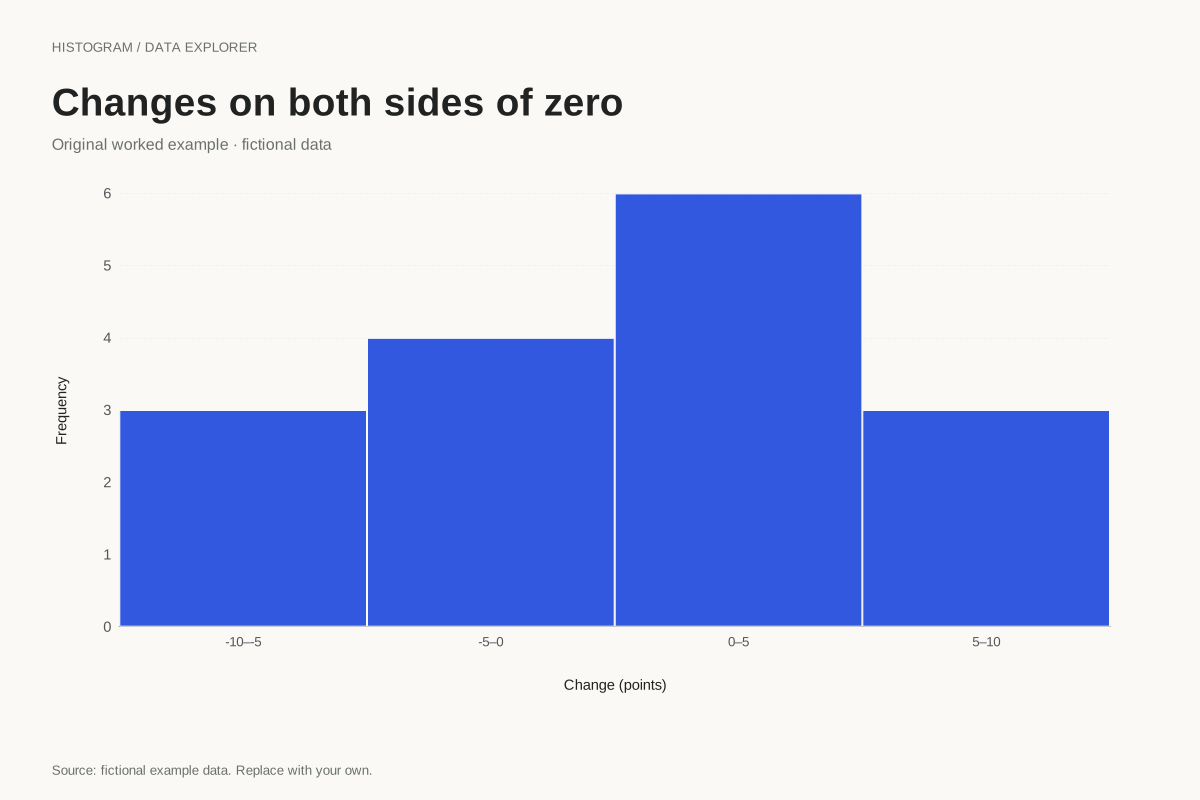
Histogram with negative and positive observations
Histograms can include values below zero. This fictional set represents signed measurement differences, grouped into equal five-unit intervals from −10 to 10. Zero is a value on the axis, not a missing-data code.
Explore chart & data