The comparison at a glance
| Statistic | Calculation | Result |
|---|---|---|
| N | Count rows | 16 |
| Sum | Add waits | 100 minutes |
| Mean | 100 / 16 | 6.25 minutes |
| Median | Average positions 8 and 9 | 4 minutes |
Calculate both from the same list
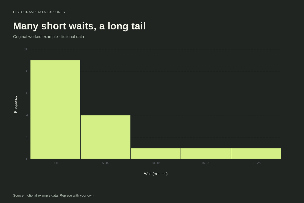
Our sixteen waiting times total 100 minutes, so their mean is 100 ÷ 16 = 6.25 minutes. The eighth and ninth sorted observations are both 4, making the median 4 minutes. Neither result is a mistake: the longer waits contribute to the sum while the median depends on central positions.
Change one value to inspect sensitivity
If the 23-minute wait became 39 minutes, the total would rise by 16 and the mean would rise by one minute to 7.25. The middle positions would remain 4 and 4, so the median would stay 4. This controlled change demonstrates sensitivity without deleting the long experience from the data.
Match the summary to the decision
For total staffing time across these observations, the sum and mean are directly connected. For the central ordered experience, the median may be useful. Neither describes the longest waits or their frequency. A histogram or dot plot alongside both summaries prevents one central number from standing in for the whole distribution.
Avoid a universal winner
The median is not automatically better whenever a histogram looks skewed. The purpose of the measurement matters, as do the sample definition and collection process. Report units, N and the population or period represented. This example is fictional and descriptive; it supports arithmetic practice, not a service benchmark or an inference about a larger population.
A related chart you can inspect
References and reproducibility
The worked arithmetic and teaching examples on this page are original. Background reading: NIST measures of location. Source code and reuse terms expose the implemented calculations.
Written by SupaMakers for ChartsAI · Reviewed September 8, 2026.