One score list, two bin widths
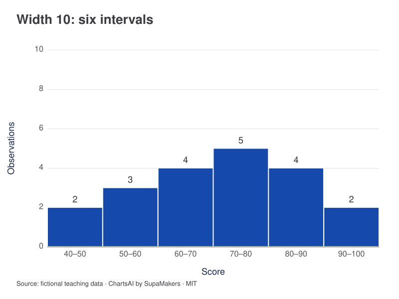
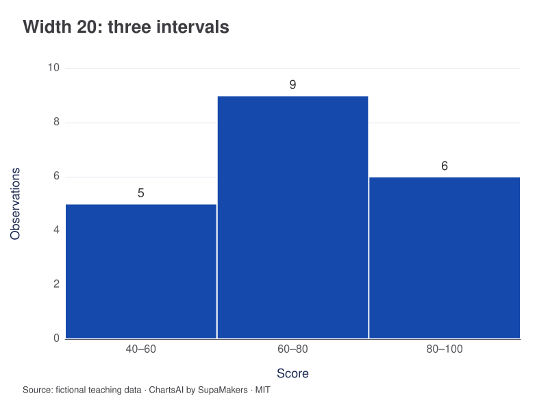
Both charts contain the same 20 scores and start at 40. Width 20 combines each adjacent pair of width-10 bins: 2 + 3 = 5, 4 + 5 = 9, and 4 + 2 = 6. Taller bars here reflect wider grouping, not additional students.
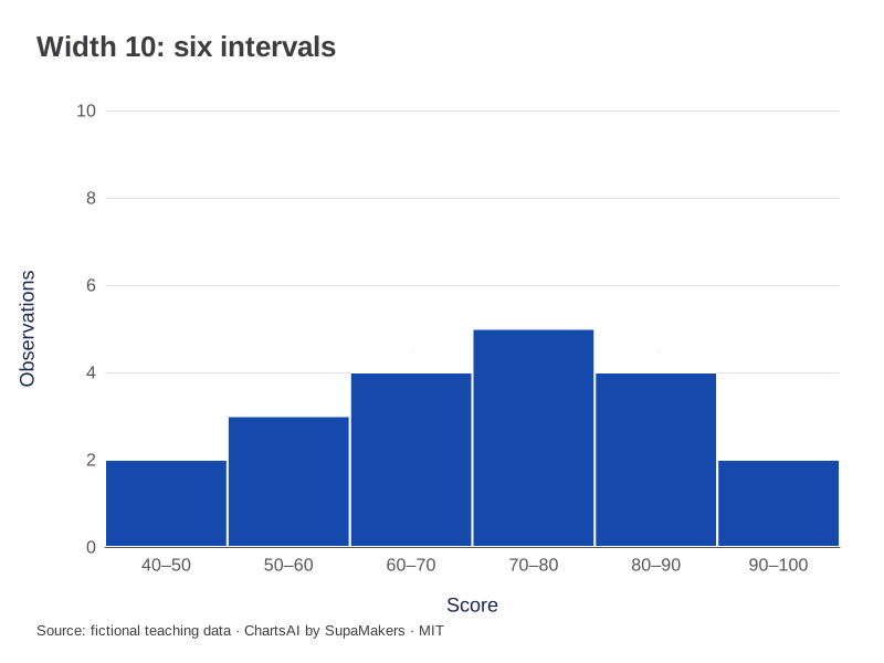
Width 10; start 40. Counts: 2, 3, 4, 5, 4, 2. N = 20.
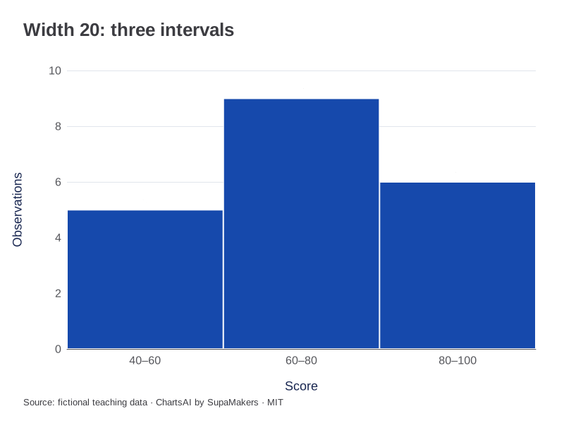
Width 20; start 40. Counts: 5, 9, 6. N = 20.
Inspect the original data and method
Counts, not density. Equal-width bins within each panel; the same start and observations across panels. Intervals include their left endpoint and exclude their right, except the final interval includes both. Both panels share a frequency axis from 0 to 10; counts grow when adjacent bins combine.
| Score |
|---|
| 42 |
| 48 |
| 52 |
| 56 |
| 58 |
| 61 |
| 63 |
| 66 |
| 68 |
| 70 |
| 72 |
| 74 |
| 76 |
| 78 |
| 81 |
| 83 |
| 85 |
| 88 |
| 92 |
| 97 |
Each CSV contains the input for that view. A box-plot CSV adds the same sample label to each observation; it does not substitute quartiles for raw values. Downloaded graphics use the same rendering specification as these previews.
The comparison at a glance
| Setting | Width 10 | Width 20 |
|---|---|---|
| Start | 40 | 40 |
| Bin count | 6 | 3 |
| Frequencies | 2, 3, 4, 5, 4, 2 | 5, 9, 6 |
| Total observations | 20 | 20 |
A width change is a data grouping change
The twenty fictional scores in our example use width 10 from a start of 40. Their counts are 2, 3, 4, 5, 4 and 2. With width 20 from the same start, adjacent counts combine into 5, 9 and 6. The observations have not changed, but the grouped description has become coarser.
Start and width work together
A width of ten beginning at 40 is not equivalent to a width of ten beginning at 35. Different boundary positions can place observations into different intervals and shift a visible peak. Report the start or full boundaries when reproducibility matters. The calculated table gives both endpoints and makes the inclusion convention explicit.
Watch for unstable stories
If a claimed cluster appears only under one carefully chosen width, inspect the raw data and alternative widths before emphasizing it. Very narrow bins in a small sample can create isolated spikes. Very wide bins can combine distinct groups. A useful choice communicates the relevant scale without pretending that a histogram is independent of its settings.
Use the controls predictably
In this maker an explicit positive bin width overrides the requested bin count. The final interval includes the maximum observation. Clearing width lets the requested count determine an equal width over the chosen range. Settings that would create more than fifty bins are rejected, so no observations disappear merely to satisfy a visual limit.
References and reproducibility
The worked arithmetic and teaching examples on this page are original. Background reading: NIST histogram background. Source code and reuse terms expose the implemented calculations.
Written by SupaMakers for ChartsAI · Reviewed September 9, 2026.